Introduction

With the developments in the field of computers, human kind has solved many problems in his life. But the revolution begins when something unique happens and i.e. what happened when mankind combined Statistics and Computer Science together, which gives birth to Machine Learning. Because of which many complex problems have been resolved too within no span of time. Machine Learning contains the specialized algorithms which let your machine iterate over a set of data for making the predictions. It basically helps us to estimate the factors like sales, growth, market evaluation, customer demand, and many more. So let’s get started with the basics of this problem-solving skill using intelligent machines by studying the Regression Models.

Learning Objectives

1. What is Regression?
2. Key Types of Regressions
3. Linear Regression Model
4. Pro and Cons of Linear Regression Model
5. Model Training and Evaluation
6. Cost Evaluation using Gradient Descent
7. Overfitting and Underfitting
8. Model Evaluation Metrics

What is Regression?

It is a statistical method that can help to analyze and understand the relationship b/w two or more variables of interest. Regression Analysis adopts the process that helps to understand which factors are mandatory, which factors can be ignored, and how these factors are influencing each other.

For the regression analysis there are two basic terms that are required to understand:

• Dependent Variable: It is the variable that we are trying to understand or forecast.
• Independent Variable: It is a variable that acts as the factor that can influence the overall analysis or target variable and provide us with information regarding the relationship of the variables with the target variable.

Key types of Regressions

There are different types of Regression Analysis techniques and these techniques can be selected on the basis of many other factors. These factors are the types of the target variable, the number of independent variables, and shape of the regression line.
Key types of regression:

1. Linear Regression
2. Logistic Regression
3. Polynomial Regression
4. Ridge Regression
5. Lasso Regression

Linear Regression Model

It is one of the most basic Regression models which contains the predictable and a dependent variable related linearly to each other. In case the data you have contains more than one independent variable, then linear regression models become the multi-linear regression model.

Equation that is used to denote the Linear Regression:

Where m is the slope of the line, c is an intercept and e is the error in the model.

(Linear Regression Example Illustration)

Pros and Cons of Regression Model

Pros of the Linear Regression model are:

1. It is really simple to implement
2. It is Highly Interpretable
3. Predictions can be done fastly
4. It is easy to train the data
5. Less resources are required to implement this model

Cons of the Linear Regression Model:

1. We made the fundamental assumption that there is a linear relationship between feature and label
2. This model doesn’t work with the outliers
3. Many features than interpretability is low
4. Categorical data is inappropriate for this model
5. Handling missing data creates problem for this model
6. Multicollinearity is a big issue

Model Training an Evaluation

We have different models, which can be developed by supplying the data to intelligent codes i.e. Algorithms which can help to learn the patterns. Then we have the Trained models with us. This whole process of supplying data to algorithms and getting the model is done under the Training Phase. Once we have our deployed Training Model, we supplied the new data (which was not used earlier) to that model so as to make the predictions.

This is how models are created and make the predictions.

Cost Evaluation using Gradient Descent

It enables a model to learn the gradient or direction that the model should take in order to reduce errors (differences between actual y and predicted y). Direction in the simple linear regression refers to how the model parameters b0 and b1 should be tweaked or corrected to further reduce the cost function. As the model iterates, it gradually converges towards a minimum where further tweaks to the parameters produce little or zero changes in the loss — also referred to as convergence.

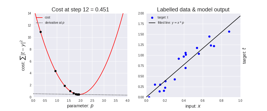
At this point, the model has optimized the weights such that they minimize the cost function. This process is integral to the ML process because it greatly expedites the learning process – you can think of it as a means of receiving corrective feedback on how to improve upon your previous performance.

Overfitting and Underfitting

Overfitting

A model is said to be overfitted, when we train it with a lot of data and now it starts learning from the noise and inaccurate data entries. Because this model does not categorize the data accurately due to many details and noise. This problem occurs when the model is too complex. In regression models, overfitting can possibly produce the R-Squared values, regression coefficients, and p-values.

In nutshell, Overfitting is the High variance and Low bias

Underfitting

A model is said to be underfitt when it cannot capture the underlying trend of data. It destroys the accuracy, as its occurrence signifies that our algorithm or model does not fit the data very well. It usually happens when we have less amount of data for training the model.

In nutshell, Underfitting is High bias and Low variance

Model Evaluation Metrics

Here are the three common model evaluation metrics for regression problems:

1. 1. Mean Absolute Error (MAE): It is the mean of absolute value of errors. It can be denoted as

MAE is the easiest to understand because it’s the average error.

1. 1. Mean Square Error (MSE): It is the mean of the squared error. It can be denoted as:

MSE is more popular than MAE, because MSE “punishes” larger errors, which tends to be useful in the real world. Also, MSE is continuous and differentiable, making it easier to use than MAE for optimization.

1. 1. Root Mean Square Error (RMSE): It is the square root of the mean of the squared root. It can be denoted as:

RMSE is even more popular than MSE, because RMSE is interpretable in the “y” units.

Are you also thinking the same that we are? Isn’t theoretical knowledge about Linear Regression quite confusing? Let’s get into the hands-on section. But for that you have to visit our detailed meetup session from here: